作为程序员,CPU在我们的工作中扮演了核心角色,因此了解处理器内部的工作方式对程序员来说不无裨益。
CPU是如何工作的呢?一条指令执行需要多长时间?当我们讨论某个新款处理器拥有12级流水线还是18级流水线,甚至是更深的31级流水线时,这到些都意味着什么呢?
应用程序通常会将CPU看作是黑盒子。程序中的指令按照顺序依次进入CPU,执行完之后再按顺序依次从CPU中出来,而内部到底发生了什么,我们通常并不了解。
对我们程序员来说,尤其是对做程序性能调优工作的程序员来说,学习CPU内部的细节非常必要。否则,如果你不知道CPU的内部结构,那如何才能针对CPU做性能优化?
本文所关注的就是专门针对X86处理器流水线的工作原理。
你需要掌握的预备知识
首先,阅读本文你需要了解编程,最好了解一点汇编语言。如果你还不知道指令指针(instruction pointer)是什么,那么本文对你来说可能有些难。你需要知道什么是寄存器,指令和缓存,如果不明白它们是什么,你需要尽快查找资料了解一下。
第二,CPU的工作原理是一个非常庞大和复杂的话题,本文仅仅是匆匆一瞥,很难以用一篇文章详尽叙述。如果我有什么疏漏,请通过评论告诉我。
第三,我仅仅关注英特尔处理器及其X86架构。当然除了X86,还有很多其他架构的处理器。虽然AMD公司引入了很多新特性到X86架构,但是X86架构是Intel公司发明,并且创造了X86指令集,其中绝大多数特性是由Intel引入的。所以为了保持叙述的简单和一致性,我仅关注Intel的处理器。
最后,当你读到这篇文章时,它已经是“过时”的了。更新款的处理器已经设计出来,其中一些会在未来几个月之内发布。我很高兴技术能如此快速的发展,我希望有一天所有这些技术都会过时,创造出拥有更惊人计算能力的CPU。
处理器流水线基础
从一个非常广的角度来说,X86处理器架构在近35年来并没有变化太多。虽然X86架构被附加了很多新功能,但是最初的设计(包括几乎所有最初的指令集)仍然基本上是完整保留的,即使在最新的处理器上仍然被支持。
最初的8086处理器支持14个寄存器,这些寄存器在如今最新的处理器中仍然存在。这14个寄存器中,有4个是通用寄存器:AX,BX,CX和DX;有4个是段寄存器,段寄存器用来辅助指针的实现:代码段(CS),数据段(DS),扩展段(ES)和堆栈段(SS);有4个是索引寄存器,用来指向内存地址:源引用(SI),目的引用(DI),基指针(BP),栈指针(SP);有1个寄存器包含状态位;最后是最重要的寄存器:指令指针(IP)。
指令指针寄存器是一个拥有特殊功能的指针。指令指针的功能是指向将要运行的下一条指令。
所有的X86处理器都按照相同的模式运行。首先,根据指令指针指向的地址取得下一条即将运行的指令并解析该指令(译码)。在译码完成后,会有一个指令的执行阶段。有些指令用来从内存读取数据或者向内存写数据,有些指令用来执行计算或者比较等工作。当指令执行完成后,这条指令会通过退出(retire)阶段并将指令指针修改为下一条指令。
译码,执行和退出三级流水线组成了X86处理器指令执行的基本模式。从最初的8086处理器到最新的酷睿i7处理器都基本遵循了这样的过程。虽然更新的处理器增加了更多的流水级,但基本的模式没有改变。
35年来发生了什么改变
相较于现今的标准,最初的处理器设计显得太过简单。最初的8086处理器的执行过程可以简述为从当前指令指针取得指令,通过译码,执行最后退出,然后继续从指令指针指向的下一条指令处取得指令。
新的处理器增加了新的功能,有些增加了新的指令,有些增加了新的寄存器。我将主要关注和本文主题有关系的改变,这些改变影响了CPU指令执行的流程。其他的一些变化比如虚拟内存或者并行处理虽然都很有意义而且有趣,但是并不在本文主题的范围内。
指令缓存在1982年被加入到处理器中。通过指令缓存,处理器可以一次性从内存读取更多指令并放在指令缓存中,而不用每条指令都从内存中取。指令缓存仅有几个字节大小,只能容纳数条指令,但是因为消除了之后每次取指往返内存和处理器的时间,极大的提高的效率
1985年的386处理器引入了数据缓存,而且扩展了指令缓存的设计。数据访存请求通过一次性读取更多的数据放在数据缓存中,从而提升了性能。而且,数据缓存和指令缓存都从几个字节扩大到几千字节。
1989年推出的i486处理器引入了五级流水线。这时,在CPU中不再仅运行一条指令,每一级流水线在同一时刻都运行着不同的指令。这个设计使得i486比同频率的386处理器性能提升了不止一倍。五级流水线中的取指阶段将指令从指令缓存中取出(i486中的指令缓存为8KB);第二级为译码阶段,将取出的指令翻译为具体的功能操作;第三级为转址阶段,用来将内存地址和偏移进行转换;第四级为执行阶段,指令在该阶段真正执行运算;第五级为退出阶段,运算的结果被写回寄存器或者内存。由于处理器同时运行了多条指令,大大提升了程序运行的性能。
1993年Intel推出了奔腾(Pentium)处理器。由于诉讼问题,Intel无法继续沿用原来的数字编号。因此,用奔腾替代了586作为新款处理器的代号。奔腾处理器相对i486处理器对流水线做出了更多修改。奔腾处理器架构增加了第二条独立的超标量流水线。主流水线工作方式类似于i486,第二条流水线则并行的运行一些较简单的指令,比如说定点算术,而且该流水线能更快的进行该运算。
1995年Intel推出了奔腾Pro(Pentium Pro)处理器。和之前的处理器相比,奔腾Pro采用了完全不同的设计。该处理器采用了诸多新特性以提高性能,包括乱序(Out-of-Order, OOO)执行的部件以及猜测执行。流水线扩展到了12级,而且引入了“超标量流水线”的概念,使得许多指令可以被同时处理。我们稍后将详尽的介绍乱序执行的部件。
在1995-2002年之间,乱序执行部件经过了数次重大改进。处理器中加入了更多的寄存器;单指令多数据(Single Instruction Multiple Data, or SIMD)的引入使得一条指令可以进行多组数据运算;现有的缓存变得更大而且引入了新的缓存;有些流水级被拆分成更多流水级,有些流水级被合并,使得更加适合实际的应用。这些改变对整体性能的提升有重要作用,但它们都没有从根本影响数据在处理器中的流动方式。
2002年发布的奔腾4处理器引入了超线程技术。乱序执行部件的设计使得指令被执行的速度比处理器能够提供指令的速度更快。因此对于大部分应用,CPU的乱序执行部件在大部分时间处于空闲状态,甚至在高负载的情况下也不能充分利用。为了让指令流能充分的流入乱序执行部件,Intel加入了第二套前端部件(译注:在处理器结构中,前端是指取指,译码,寄存器重命名等模块,经过前端部件的处理后,指令等待发射进入乱序执行部件)。虽然实际上只有一个乱序执行部件,但对于操作系统来说,它能看到两个处理器。前端部件包含两组同样功能的X86寄存器,两个指令译码器根据两个指令指针指向的地址分别处理。所有的指令被一个共享的乱序执行部件执行,但对应用程序来说并不知情。当乱序执行部件执行完成,像之前一样退出流水线后,最终结果返回虚拟的两个处理器。
2006年Intel发布了酷睿(Core)微架构。为了品牌效应,它被称做酷睿2(二总比一好)。令人惊讶的是,处理器频率不升反降,而且超线程也被去掉了。通过降低时钟频率,每一级流水线可以做更多工作。乱序执行部件也被扩展的更宽。各种不同的缓存和队列都相应做的更大。而且处理器被重新设计,以适应双核和四核的共享缓存结构。
2008年,Intel开始用酷睿i3, i5, i7的方式来命名新的处理器。新处理器重新引入了超线程。这三个系列的处理器主要区别在于内部缓存大小不同。
未来的处理器:Intel的下一代微结构被称为Haswell。Haswell据称将于2013年发布。目前已知的文档说明它将拥有14级流水级的乱序执行部件,所以它仍然遵循从奔腾Pro以来的基本设计思路。
那么,流水线到底是什么?乱序执行部件是什么?他们如何提升了处理器的性能呢?
CPU指令流水线
根据之前描述的基础,指令进入流水线,通过流水线处理,从流水线出来的过程,对于我们程序员来说,是比较直观的。
I486拥有五级流水线。分别是:取指(Fetch),译码(D1, main decode),转址(D2, translate),执行(EX, execute),写回(WB)。某个指令可以在流水线的任何一级。

但是这样的流水线有一个明显的缺陷。对于下面的指令代码,它们的功能是将两个变量的内容进行交换。

从8086直到386处理器都没有流水线。处理器一次只能执行一条指令。再这样的架构下,上面的代码执行并不会存在问题。
但是i486处理器是首个拥有流水线的x86处理器,它执行上面的代码会发生什么呢?当你一下去观察很多指令在流水线中运行,你会觉得混乱,所以你需要回头参考上面的图。
第一步是第一条指令进入取指阶段;然后在第二步第一条指令进入译码阶段,同时第二条指令进入取指阶段;第三步第一条指令进入转址阶段,第二条指令进入译码阶段,第三条指令进入取指阶段。但是在第四步会出现问题,第一条指令会进入执行阶段,而其他指令却不能继续向前移动。第二条xor指令需要第一条xor指令计算的结果a,但是直到第一条指令执行完成才会写回。所以流水线的其他指令就会在当前流水级等待直到第一条指令的执行和写回阶段完成。第二条指令会等待第一条指令完成才能进入流水线下一级,同样第三条指令也要等待第二条指令完成。
这个现象被称为流水线阻塞或者流水线气泡。
另外一个关于流水线的问题是有些指令执行速度快,有些指令执行速度慢。这个问题在奔腾处理器的双流水线架构下显得更加明显。
奔腾Pro拥有12级流水线。当这个数字被首次宣布后,所有的程序员都倒抽了一口气,因为他们知道超标量流水线是如何工作的。如果Intel仍然按照以前的思路设计超标量流水线的话,流水线的阻塞和执行速度慢的指令会严重影响执行速度。但同时,Intel宣布了完全不同的流水线设计,叫做乱序执行部件(Out-of-Order core)。单从叙述上很难理解这些改变带来的好处,但Intel确信这些改进是令人激动的。
让我们来更深入的看看这个乱序执行的部件吧!
乱序执行流水线
在描述乱序执行流水线时,往往是一图胜千言。所以我们主要以图例进行介绍。
CPU流水线图例
I486处理器拥有5级流水线。这种设计在现实世界中的其他处理器中很常见,而且效率不错。

而奔腾处理器的流水线比i486更好。两条流水线可以并行运行,而且每条流水线可以同时有多条指令在不同流水级执行。它几乎可以同时执行比i486多一倍的指令。

能够快速完成的指令需要等待前面执行慢的指令即使在并行流水线中也仍然是一个问题。流水线仍然是线性的,导致处理器面临性能瓶颈难以逾越。
乱序执行部件和之前处理器设计中的线性通路有很大不同,它增加了一些复杂度,引入了非线性的通路。

第一个改变是指令从内存中取到处理器的指令缓存的过程。现代处理器能够检测何时会产生一个大的分支跳转(比如函数调用),然后提前将跳转目的地的指令加载到指令缓存中。
译码级有一些略微的修改。不同于以往处理器仅仅译码指令指针指向的指令,奔腾Pro处理器每一个始终周期最多能译码3条指令。现今的处理器(2008-2013年)每个时钟周期最多可以译码4条指令。译码过程产生很多小片的操作,被称作微指令(micro-ops, ?-ops)。
下一级(或者好几级)被称为微指令翻译,接着是寄存器重命名(register aliasing)。许多操作同时执行,并且执行的顺序是乱序的,所以有可能出现一条指令读一个寄存器的同时,另外一条指令正在对这个寄存器进行写操作。在处理器内部,这些原始的寄存器(如AX,BX,CX,DX等)被翻译(或者重命名)成为内部的寄存器,而这些寄存器对程序员是不可见的。寄存器和内存地址需要被映射到一个临时的地方用于指令执行。当前每个始终周期可以翻译4条微指令。
当微指令翻译完成后,它们会进入一个重排序缓存(Reorder Buffer, ROB),ROB可以存储最多128条微指令。在支持超线程的处理器上,ROB同样可以重排来自两个虚拟处理器的指令。两个虚拟处理器在ROB中将微指令汇集到一个共享的乱序执行部件中。
这些微指令已经准备好可以执行了。它们被放在保留站中(Reservation Station, RS)。RS最多可以同时存储36条微指令。
现在才开始乱序执行部件神奇的部分。不同的微指令在不同的执行单元中同时执行,而且每个执行单元都全速运行。只要当前微指令所需要的数据就绪,而且有空闲的执行单元,微指令就可以立即执行,有时甚至可以跳过前面还未就绪的微指令。通过这种方式,需要长时间运行的操作不会阻塞后面的操作,流水线阻塞带来的损失被极大的减小了。
奔腾Pro的乱序执行部件拥有6个执行单元:两个定点处理单元,一个浮点处理单元,一个取数单元,一个存地址单元,一个存数单元。这两个定点处理单元有所不同,一个能够处理复杂定点操作,一个能同时处理两个简单操作。在理想状况下,奔腾Pro的乱序执行部件可以在一个时钟周期内执行7条微指令。
现今的乱序执行部件仍然拥有6个执行单元。其中取数单元,存地址单元,存数单元没有变,另外3个多少发生了变化。这三个执行单元都可以执行基本算术运算,或者执行更复杂的微指令。但每个执行单元擅长执行不同种类的微指令,使得它们能更高效的执行运算。在理想状况下,现今的乱序执行部件可以在一个时钟周期内执行11条微指令。
最终微指令会得到执行,在经过数个流水级之后,最终会退出流水线。这时,这条指令完成并且递增指令指针。但从程序员的角度来说,指令仅仅是从一端进入CPU,从另一端退出,就像老的8086一样。
如果你仔细看过上面的内容,你会注意到上面提到过很重要的一个问题:如果执行指令的位置发生了跳转会发生什么?例如,当指令运行到”if”或者是”switch”时,会发生什么呢?在较老的处理器中这意味着清空流水线,等待新的跳转目的指令的取指执行。
当CPU指令队列中存储了超过100条指令时,发生流水线阻塞带来的性能损失是极其严重的。所有的指令都需要等待跳转目的的指令取回并且重启流水线。在这种情况下,乱序执行部件需要将跳转指令之后但是已经执行的微指令全部取消掉,返回到执行前的状态。当所有乱序执行的微指令都退出乱序执行部件之后,将它们丢弃掉,然后从新的地址开始执行。这对于处理器来说是相当困难的,而且发生的频率很高,因此对性能的影响很大。这时,引入了乱序执行部件的另外一个重要功能。
答案就是猜测执行。猜测执行意味着当遇到一个分支指令后,乱序执行部件会将所有分支的指令都执行一遍。一旦分支指令的跳转方向确定后,错误跳转方向的指令都将被丢弃。通过同时执行两个跳转方向的指令,避免了由于分支跳转导致的阻塞。处理器设计者还发明了分支预测缓存,当面临多个分支时进行预测,进一步提高了性能。虽然CPU阻塞仍然会发生,但是这个解决方案将CPU发生阻塞的概率降到了一个可以接受的范围。
最后,拥有超线程的处理器将两个虚拟的处理器暴露给共享的乱序执行部件。它们共享一个重排序缓存和乱序执行部件,让操作系统认为它们是两个独立的处理器,看上去就像这样:

超线程的处理器拥有两个虚拟的处理器,从而可以给乱序执行部件提供更多的数据。超线程对一般的应用程序都有性能提升,但是对一些计算密集型的应用,则会迅速使得乱序执行部件饱和。在这种情况下,超线程反而会略微降低性能。但这种情况毕竟是少数,超线程对于日常应用来讲通常都能够提供大约一倍的性能。
一个示例
这一切看上去有点令人感到困惑,那么我们举一个例子来让这一切变得清晰起来。
从应用程序的角度来看,我们仍然是运行在指令流水线上,就想老的8086处理器那样。处理器就是一个黑盒子。黑盒子会处理指令指针指向的指令,当处理完之后,会在内存里找到处理的结果。
但是从指令本身的角度来讲,这个过程可谓历经沧桑。我们下面介绍对于现今的处理器(大约在2008-2013年之间),一条指令在其内部的过程。
首先,你是一条指令,你所属的程序正在运行。
你一直在耐心的等待指令指针会指向自己,等待被CPU运行。当指令指针距离你还有4KB远的时候(这大约是1500条指令),你被CPU从内存取到指令缓存中。虽然从内存加载进入指令缓存需要一段时间,但是现在距离你被执行的时刻还很远,你有足够的时间。这个预取的过程属于流水线的第一级。
当指令指针离你越来越近,距离你还有24条指令的时候,你和你旁边的5个指令会被放到指令队列里面。
这个处理器有4个译码器,可以容纳一个复杂指令和最多三个简单指令。你碰巧是一条复杂指令,通过译码,你被翻译成4个微指令。
译码的过程可以划分为多步。译码过程中的一步是检查你需要的数据和猜测你可能会产生一个地址跳转。译码器一旦检测到需要的额外数据,不需要让你知道,这个数据就开始从内存加载到数据缓存中了。
你的四个微指令到达寄存器重命名表。你告诉它你需要读哪个内存地址(比如说fs:[eax+18h]),然后寄存器重命名表将这个地址转换为临时地址供微指令使用。地址转化完成后,你的微指令将进入重排序缓存(Reorder Buffer, ROB)并记录指令次序。接着第一时间进入保留站(Reservation Station, RS)。
保留站用于存储已经准备就绪可以执行的指令。你的第三条微指令被立即选中并送往端口5,这个端口直接执行运算。但是你并不知道为什么它会被首先选中,无论如何,它确实被执行了。几个时钟周期之后你的第一条微指令前往端口2,该端口是读单元(Load Address execution unit)。剩余的微指令一直等待,同时各个端口正在收集不同的微指令。他们都在等待端口2将数据从缓存和内存中加载进来并放在临时存储空间内。
他们等了很久……
相当久的时间……
不过在他们等待第一条微指令返回数据的时候,又有其他的新指令又进来。好在处理器知道如何让这些指令乱序执行(即后到达保留站的微指令被优先执行)。
当第一条微指令返回了数据,剩余的两条微指令被立即送往执行端口0和1。现在这4条微指令都已经运行,最终它们会返回保留站。
这些微指令返回后交出他们的“票”并给出各自的临时地址。通过这些地址,你作为一个完整的指令,将他们合并。最后CPU将结果交给你并使你退出
当你到达标有“退出”的门的时候,你会发现这里要排一个队列。你进入后发现你刚好站在你前面进来指令的后面,即使执行中的顺序可能已经不同,但你们退出的顺序继续保持一致。看来乱序执行部件真正知道自己做了什么。
每条指令最终离开CPU,每次一条指令,就和指令指针指向的顺序一样!
结论
希望这篇小文能够给读者展示一些处理器工作的奥秘,要知道,这并不是魔术。
让我们回到最初的问题,现在我们应该可以给出一些较好的答案了。
处理器内部是如何工作的呢?在这个复杂的过程中,指令首先被分解为更小的微指令命令,这些微指令以乱序的方式尽可能快的被执行,然后按照原始的顺序提交执行结果。因此,从外部看来,所有的指令都是按照顺序的方式执行的。但是现在我们知道,处理器内部是以乱序的方式处理指令的,有时甚至以猜测的方式来运行分支代码。
运行一条指令究竟需要多长时间呢?对于没有使用流水线技术的处理器来说,这是一个容易回答的问题,但对于现代的处理器来说,一条指令的执行时间与它周围指令的内容以及临近cache的大小和内容都有关。一条指令通过处理器有一个最小的时间,但只能粗略的说这个时间是恒定的。一个好的程序员和编译器可以让很多条指令同时运行,从而使每条指令的分摊时间几乎为零。这里说的几乎为零的执行时间并不是指一条指令的总的执行时间很短,相反,通过整个乱序部件和等待内存读写数据是需要花费很多时间的。
一个新的处理器拥有12级或者18级、甚至更深的31级流水线意味着什么呢?这意味着更多的指令可以被同时送进加工厂。一个非常深的流水线可以让几百条指令同时被处理。当一切顺利时,一个乱序部件可以保持高速运转,从而获得惊人的吞吐量。不幸的是,深的流水线同时意味着流水线停顿会从一个相对可以容忍的性能损失变成一个可怕的性能噩梦。因为几百条指令都不得不停顿下来,等待流水线恢复运转。
我怎么根据这些信息来优化程序呢?幸运的是,CPU可以在大部分常见情况下工作良好,并且编译器已经为乱序处理器优化了近20年。当指令和数据按照顺序(没有烦人的跳转)执行时,CPU可以获得最好的性能。因此,首先,使用简单的代码。简单直接的代码会帮助编译器的优化引擎识别并优化代码。尽量不使用跳转指令,当你不得不跳转时,尽量每次跳转到同样的方向。复杂的设计,例如动态跳转表,虽然看起来很酷并且的确可以完成非常强大的功能,但不管是处理器还是编译器,都无法进行很好的预测处理,因此复杂的代码很可能导致流水线停顿和猜测错误,从而极大的损害处理器性能。其次,使用简单的数据结构。保持数据顺序、相邻和连续可以阻止数据停顿。使用正确的数据结构和数据分布可以获得很大的性能提升。只要保持代码和数据结构尽量简单,剩下的工作就可以放心地交给编译器的优化引擎来完成了。
感谢与我一起参与这次旅行!
附原文:
What goes on inside the CPU? How long does it take for one instruction to run? What does it mean when a new CPU has a 12-stage pipeline, or 18-stage pipeline, or even a “deep” 31-stage pipeline?
Programs generally treat the CPU as a black box. Instructions go into the box in order, instructions come out of the box in order, and some processing magic happens inside.
As a programmer, it is useful to learn what happens inside the box. This is especially true if you will be working on tasks like program optimization. If you don’t know what is going on inside the CPU, how can you optimize for it?
This article is about what goes on inside the x86 processor’s deep pipeline.
Stuff You Should Already Know
First, this article assumes you know a bit about programming, and maybe even a little assembly language. If you don’t know what I mean when I mention an instruction pointer, this article probably isn’t for you. When I talk about registers, instructions, and caches, I assume you already know what they mean, can figure it out, or will look it up.
Second, this article is a simplification of a complex topic. If you feel I have left out important details, please add them to the comments at the end.
Third, I am focusing on Intel processors and the x86 family. I know there are many different processor families out there other than x86. I know that AMD introduced many useful features into the x86 family and Intel incorporated them. It is Intel’s architecture and Intel’s instruction set, and Intel introduced the most major feature being covered, so for simplicity and consistency I’m just going to stick with their processors.
Fourth, this article is already out of date. Newer processors are in the works and some are due out in a few months. I am very happy that technology is advancing at a rapid pace. I hope that someday all of these steps are completely outdated, replaced with even more amazing advances in computing power.
The Pipeline Basics
From an extremely broad perspective the x86 processor family has not changed very much over its 35 year history. There have been many additions but the original design (and nearly all of the original instruction set) is basically intact and visible in the modern processor.
The original 8086 processor has 14 CPU registers which are still in use today. Four are general purpose registers — AX, BX, CX, and DX. Four are segment registers that are used to help with pointers — Code Segment (CS), Data Segment (DS), Extra Segment (ES), and Stack Segment (SS). Four are index registers that point to various memory locations — Source Index (SI), Destination Index (DI), Base Pointer (BP), and Stack Pointer (SP). One register contains bit flags. And finally, there is the most important register for this article: The Instruction Pointer (IP).
The instruction pointer register is a pointer with a special job. The instruction pointer’s job is to point to the next instruction to be run.
All processors in the x86 family follow the same pattern. First, they follow the instruction pointer and decode the next CPU instruction at that location. After decoding, there is an execute stage where the instruction is run. Some instructions read from memory or write to it, others perform calculations or comparisons or do other work. When the work is done, the instruction goes through a retire stage and the instruction pointer is modified to point to the next instruction.
This decode, execute, and retire pipeline pattern applies to the original 8086 processor as much as it applies to the latest Core i7 processor. Additional pipeline stages have been added over the years, but the pattern remains.
What Has Changed Over 35 Years
The original processor was simple by today’s standard. The original 8086 processor began by evaluating the instruction at the current instruction pointer, decoded it, executed it, retired it, and moved on to the next instruction that the instruction pointer pointed to.
Each new chip in the family added new functionality. Most chips added new instructions. Some chips added new registers. For the purposes of this article I am focusing on the changes that affect the main flow of instructions through the CPU. Other changes like adding virtual memory or parallel processing are certainly interesting and useful, but not applicable to this article.
In 1982 an instruction cache was added to the processor. Instead of jumping out to memory at every instruction, the CPU would read several bytes beyond the current instruction pointer. The instruction cache was only a few bytes in size, just large enough to fetch a few instructions, but it dramatically improved performance by removing round trips to memory every few cycles.
In 1985, the 386 added cache memory for data as well as expanding the instruction cache. This gave performance improvements by reading several bytes beyond a data request. By this point both the instruction cache and data cache were measured in kilobytes rather than bytes.
In 1989, the i486 moved to a five-stage pipeline. Instead of having a single instruction inside the CPU, each stage of the pipeline could have an instruction in it. This addition more than doubled the performance of a 386 processor of the same clock rate. The fetch stage extracted an instruction from the cache. (The instruction cache at this time was generally 8 kilobytes.) The second stage would decode the instruction. The third stage would translate memory addresses and displacements needed for the instruction. The fourth stage would execute the instruction. The fifth stage would retire the instruction, writing the results back to registers and memory as needed. By allowing multiple instructions in the processor at once, programs could run much faster.
1993 saw the introduction of the Pentium processor. The processor family changed from numbers to names as a result of a lawsuit?that’s why it is Pentium instead of the 586. The Pentium chip changed the pipeline even more than the i486. The Pentium architecture added a second separate superscalar pipeline. The main pipeline worked like the i486 pipeline, but the second pipeline ran some simpler instructions, such as direct integer math, in parallel and much faster.
In 1995, Intel released the Pentium Pro processor. This was a radically different processor design. This chip had several features including out-of-order execution processing core (OOO core) and speculative execution. The pipeline was expanded to 12 stages, and it included something termed a ‘superpipeline’ where many instructions could be processed simultaneously. This OOO core will be covered in depth later in the article.
There were many major changes between 1995 when the OOO core was introduced and 2002 when our next date appears. Additional registers were added. Instructions that processed multiple values at once (Single Instruction Multiple Data, or SIMD) were introduced. Caches were introduced and existing caches enlarged. Pipeline stages were sometimes split and sometimes consolidated to allow better use in real-world situations. These and other changes were important for overall performance, but they don’t really matter very much when it comes to the flow of data through the chip.
In 2002, the Pentium 4 processor introduced a technology called Hyper-Threading. The OOO core was so successful at improving processing flow that it was able to process instructions faster than they could be sent to the core. For most users the CPU’s OOO core was effectively idle much of the time, even under load. To help give a steady flow of instructions to the OOO core they attached a second front-end. The operating system would see two processors rather than one. There were two sets of x86 registers. There were two instruction decoders that looked at two sets of instruction pointers and processed both sets of results. The results were processed by a single, shared OOO core but this was invisible to the programs. Then the results were retired just like before, and the instructions were sent back to the two virtual processors they came from.
In 2006, Intel released the “Core” microarchitecture. For branding purposes, it was called “Core 2” (because everyone knows two is better than one). In a somewhat surprising move, CPU clock rates were reduced and Hyper-Threading was removed. By slowing down the clock they could expand all the pipeline stages. The OOO core was expanded. Caches and buffers were enlarged. Processors were re-designed focusing on dual-core and quad-core chips with shared caches.
In 2008, Intel went with a naming scheme of Core i3, Core i5, and Core i7. These processors re-introduced Hyper-Threading with a shared OOO core. The three different processors differed mainly by the size of the internal caches.
Future Processors: The next microarchitecture update is currently named Haswell and speculation says it will be released late in 2013. So far the published docs suggest it is a 14-stage OOO core pipeline, so it is likely the data flow will still follow the basic design of the Pentium Pro.
So what is all this pipeline stuff, what is the OOO core, and how does it help processing speed?
CPU Instruction Pipelines
In the most basic form described above, a single instruction goes in, gets processed, and comes out the other side. That is fairly intuitive for most programmers.
The i486 has a 5-stage pipeline. The stages are ? Fetch, D1 (main decode), D2 (secondary decode, also called translate), EX (execute), WB (write back to registers and memory). One instruction can be in each stage of the pipeline.

There is a major drawback to a CPU pipeline like this. Imagine the code below. Back before CPU pipelines the following three lines were a common way to swap two variables in place.
XOR a, b
XOR b, a
XOR a, b
The chips starting with the 8086 up through the 386 did not have an internal pipeline. They processed only a single instruction at a time, independently and completely. Three consecutive XOR instructions is not a problem in this architecture.
We’ll consider what happens in the i486 since it was the first x86 chip with an internal pipeline. It can be a little confusing to watch many things in motion at once, so you may want to refer back to the diagram above.
The first instruction enters the Fetch stage and we are done with that step. On the next step the first instruction moves to D1 stage (main decode) and the second instruction is brought into fetch stage. On the third step the first instruction moves to D2 and the second instruction gets moved to D1 and another is fetched. On the next stage something goes wrong. The first instruction moves to EX … but other instructions do not advance. The decoder stops because the second XOR instruction requires the results of the first instruction. The variable (a) is supposed to be used by the second instruction, but it won’t be written to until the first instruction is done. So the instructions in the pipeline wait until the first instruction works its way through the EX and WB stages. Only after the first instruction is complete can the second instruction make its way through the pipeline. The third instruction will similarly get stuck, waiting for the second instruction to complete.
This is called a pipeline stall or a pipeline bubble.
Another issue with pipelines is some instructions could execute very quickly and other instructions would execute very slowly. This was made more visible with the Pentium’s dual-pipeline system.
The Pentium Pro introduced a 12-stage pipeline. When that number was first announced there was a collective gasp from programmers who understood how the superscalar pipeline worked. If Intel followed the same design with a 12-stage superscalar pipeline then a pipeline stall or slow instruction would seriously harm execution speed. At the same time they announced a radically different internal pipeline, calling it the Out Of Order (OOO) core. It was difficult to understand from the documentation, but Intel assured developers that they would be thrilled with the results.
Let’s have a look at this OOO core pipeline in more depth.
The Out Of Order Core Pipeline
The OOO Core pipeline is a case where a picture is worth a thousand words. So let’s get some pictures.
Diagrams of CPU Pipelines
The i486 had a 5-stage pipeline that worked well. The idea was very common in other processor families and works well in the real world.

The Pentium pipeline was even better than the i486. It had two instruction pipelines that could run in parallel, and each pipeline could have multiple instructions in different stages. You could have nearly twice as many instructions being processed at the same time.

Having fast instructions waiting for slow instructions was still a problem with parallel pipelines. Having sequential instruction order was another issue thanks to stalls. The pipelines are still linear and can face a performance barrier that cannot be breached.
The OOO core is a huge departure from the previous chip designs with their linear paths. It added some complexity and introduced nonlinear paths:

The first thing that happens is that instructions are fetched from memory into the processor’s instruction cache. The decoder on the modern processors can detect when a large branch is about to happen (such as a function call) and can begin loading the instructions before they are needed.
The decoding stage was modified slightly from earlier chips. Instead of just processing a single instruction at the instruction pointer, the Pentium Pro processor could decode up to three instructions per cycle. Today’s (circa 2008-2013) processors can decode up to four instructions at once. Decoding produces small fragments of operations called micro-ops or ?-ops.
Next is a stage (or set of stages) called micro-op translation, followed by register aliasing. Many operations are going on at once and we will potentially be doing work out of order, so an instruction could read to a register at the same time another instruction is writing to it. Writing to a register could potentially stomp on a value that another instruction needs. Inside the processor the original registers (such as AX, BX, CX, DX, and so on) are translated (or aliased) into internal registers that are hidden from the programmer. The registers and memory addresses need to have their values mapped to a temporary value for processing. Currently 4 micro-ops can go through translation every cycle.
After micro-op translation is complete, all of the instruction’s micro-ops enter a reorder buffer, or ROB. The ROB currently holds up to 128 micro-ops. On a processor with Hyper-Threading the ROB can also coordinate entries from multiple virtual processors. Both virtual processors come together into a single OOO core at the ROB stage.
These micro-ops are now ready for processing. They are placed in the Reservation Station (RS). The RS currently can hold 36 micro-ops at any one time.
Now the magic of the OOO core happens. The micro-ops are processed simultaneously on multiple execution units, and each execution unit runs as fast as it can. Micro-ops can be processed out of order as long as their data is ready, sometimes skipping over unready micro-ops for a long time while working on other micro-ops that are ready. This way a long operation does not block quick operations and the cost of pipeline stalls is greatly reduced.
The original Pentium Pro OOO core had six execution units: two integer processors, one floating-point processor, a load unit, a store address unit, and a store data unit. The two integer processors were specialized; one could handle the complex integer operations, the other could solve up to two simple operations at once. In an ideal situation the Pentium Pro OOO Core execution units could process seven micro-ops in a single clock cycle.
Today’s OOO core still has six execution units. It still has the load address, store address, and store data execution units, the other three have changed somewhat. Each of the three execution units perform basic math operations, or instead they perform a more complex micro-op. Each of the three execution units are specialized to different micro-ops allowing them to complete the work faster than if they were general purpose. In an ideal situation today’s OOO core can process 11 micro-ops in a single cycle.
Eventually the micro-op is run. It goes through a few more small stages (which vary from processor to processor) and eventually gets retired. At this point it is returned back to the outside world and the instruction pointer is advanced. From the program’s point of view the instruction has simply entered the CPU and exited the other side in exactly the same way it did back on the old 8086.
If you were following carefully you may have noticed one very important issue in the way it was just described. What happens if there is a change in execution location? For example, what happens when the code hits an ’if’ statement or a ’switch” statement? On the older processors this meant discarding the work in the superscalar pipeline and waiting for the new branch to begin processing.
A pipeline stall when the CPU holds one hundred instructions or more is an extreme performance penalty. Every instruction needs to wait while the instructions at the new location are loaded and the pipeline restarted. In this situation the OOO core needs to cancel work in progress, roll back to the earlier state, wait until all the micro-ops are retired, discard them and their results, and then continue at the new location. This was a very difficult problem and happened frequently in the design. The performance of this situation was unacceptable to the engineers. This is where the other major feature of the OOO core comes in.
Speculative execution was their answer. Speculative execution means that when a conditional statement (such as an ’if’ block) is encountered the OOO core will simply decode and run all the branches of the code. As soon as the core figures out which branch was the correct one, the results from the unused branches would be discarded. This prevents the stall at the small cost of running the code inside the wrong branch. The CPU designers also included a branch prediction cache which further improved the results when it was forced to guess at multiple branch locations. We still have CPU stalls from this problem, but the solutions in place have reduced it to the point where it is a rare exception rather than a usual condition.
Finally, CPUs with Hyper-Threading enabled will expose two virtual processors for a single shared OOO core. They share a Reorder Buffer and OOO core, appearing as two separate processors to the operating system. That looks like this:

A processor with Hyper-Threading gives two virtual processors which in turn gives more data to the OOO core. This gives a performance increase during general workloads. A few compute-intensive workflows that are written to take advantage of every processor can saturate the OOO core. During those situations Hyper-Threading can slightly decrease overall performance. Those workflows are relatively rare; Hyper-Threading usually provides consumers with approximately double the speed they would see for their everyday computer tasks.
An Example
All of this may seem a little confusing. Hopefully an example will clear everything up.
From the application’s perspective, we are still running on the same instruction pipeline as the old 8086. There is a black box. The instruction pointed to by the instruction pointer is processed by the black box, and when it comes out the results are reflected in memory.
From the instruction’s point of view, however, that black box is quite a ride.
Here is today’s (circa 2008-2013) CPU ride, as seen by an instruction:
First, you are a program instruction. Your program is being run.
You are waiting patiently for the instruction pointer to point to you so you can be processed. When the instruction pointer gets about 4 kilobytes away from you — about 1500 instructions away — you get collected into the instruction cache. Loading into the cache takes some time, but you are far away from being run. This prefetch is part of the first pipeline stage.
The instruction pointer gets closer and closer. When the instruction pointer gets about 24 instructions away, you and five neighbors get pulled into the instruction queue.
This processor has four decoders. It has room for one complex instruction and up to three simple instructions. You happen to be a complex instruction and are decoded into four micro-ops.
Decoding is a multi-step process. Part of the decode process involved a scan to see what data you need and if you are likely to cause a jump to somewhere new. The decoder detected a need for some additional data. Unknown to you, somewhere on the far side of the computer, your data starts getting loaded into the data cache.
Your four micro-ops step up to the register alias table. You announce which memory address you read from (it happens to be fs:[eax+18h]) and the chip translates that into temporary addresses for your micro-ops. Your micro-ops enter the reorder buffer, or ROB. At the first available opportunity they move to the Reservation Station.
The Reservation Station holds instructions that are ready to be run. Your third micro-op is immediately picked up by Execution Port 5. You don’t know why it was selected first, but it is gone. A few cycles later your first micro-op rushes to Port 2, the Load Address execution unit. The remaining micro-ops wait as various ports collect other micro-ops. They wait as Port 2 loads data from the memory cache and puts it in temporary memory slots.
They wait a long time…
A very long time…
Other instructions come and go while they wait for their micro-op friend to load the right data. Good thing this processor knows how to handle things out of order.
Suddenly both of the remaining micro-ops are picked up by Execution Ports 0 and 1. The data load must be complete. The micro-ops are all run, and eventually the four micro-ops meet back in the Reservation Station.
As they travel back through the gate the micro-ops hand in their tickets listing their temporary addresses. The micro-ops are collected and joined, and you, as an instruction, feel whole again. The CPU hands you your result, and gently directs you to the exit.
There is a short line through a door marked “Retirement”. You get in line, and discover you are standing next to the same instructions you came in with. You are even standing in the same order. It turns out this out-of-order core really knows its business.
Each instruction then goes out of the CPU, seeming to exit one at a time, in the same order they were pointed to by the instruction pointer.
Conclusion
This little lecture has hopefully shed some light on what happens inside a CPU. It isn’t all magic, smoke, and mirrors.
Getting back to the original questions, we now have some good answers.
What goes on inside the CPU? There is a complex world where instructions are broken down into micro-operations, processed as soon as possible in any order, then put back together in order and in place. To an outsider it looks like they are being processed sequentially and independently. But now we know that on the inside they are handled out of order, sometimes even running braches of code based on a prediction that they will be useful.
How long does it take for one instruction to run? While there was a good answer to this in the non-pipelined world, in today’s processors the time it takes is based on what instructions are nearby, and the size and contents of the neighboring caches. There is a minimum amount of time it takes to go through the processor, but that is roughly constant. A good programmer and optimizing compiler can make many instructions run in around amortized zero time. With an amortized zero time it is not the cost of the instruction that is slow; instead it means it takes the time to work through the OOO core and the time to wait for cache memory to load and unload.
What does it mean when a new CPU has a 12-stage pipeline, or 18-stage, or even a “deep” 31-stage pipeline? It means more instructions are invited to the party at once. A very deep pipeline can mean that several hundred instructions can be marked as ’in progress’ at once. When everything is going well the OOO core is kept very busy and the processor gains an impressive throughput of instructions. Unfortunately, this also means that a pipeline stall moves from being a mild annoyance like it was in the early days, to becoming a performance nightmare as hundreds of instructions need to wait around for the pipeline to clear out.
How can I apply this to my programs? The good news is that CPUs can anticipate most common patterns, and compilers have been optimizing for OOO core for nearly two decades. The CPU runs best when instructions and data are all in order. Always keep your code simple. Simple and straightforward code will help the compiler’s optimizer identify and speed up the results. Don’t jump around if you can help it, and if you need to jump, try to jump around exactly the same way every time. Complex designs like dynamic jump tables are fancy and can do a lot, but neither the compiler or CPU will predict what will be coming up, so complex code is very likely to result in stalls and mis-predictions. On the other side, keep your data simple. Keep your data in order, adjacent, and consecutive to prevent data stalls. Choosing the right data structures and data layouts can do much to encourage good performance. As long as you keep your code and data simple you can generally rely on your compiler’s optimizer to do the rest.
Thanks for joining me on the ride.
updates
2013-05-17 Removed a word that someone was offended by
License
GDOL (Gamedev.net Open License)
英文原文:gamedev.net,编译:感谢@deuso_ICT 的热心翻译
source:http://blog.jobbole.com/40844/